
Calculating the reachability of Metro stations in Milan
Some time ago I saw a reddit post on r/milano presenting a visualization of the nearest Metro or train station in the city of Milan. In short, it indicates for each station which area is “covered” by it, having it as the closest station.
That visualization uses Voronoi cells built with the Metro stations as the centers, and the distance metric is then the geodesic distance (“as the crow flies”), but if a station is easy to reach by tram or, on the other side, is surrounded by railways or highways making crossing difficult this distance will not represent well how “reachable” the station is by someone walking or using the tram.
I wondered then about creating a similar map but using travel times instead. Another question I had, looking at the map, is how well served different areas are in relation to the population. There’s a single station, Abbiategrasso, covering a large area in the south. It looks like that area is not well served, but I know it’s not densely populated.
In this article I’ll explain in detail how I built such a map using the road network and transit data and the intersting details of the process.
The input data
We need two sources for this kind of operation: the road network and public transport schedules.
For the road network we can use OpenStreetMap, there are services like the excellent Geofabrik providing extracts of the data for specific areas.
This data is in PBF (Protobuf) format (stricly speaking it’s based on Protobuf), and I’ve written several articles about importing it in a database. If you are curious, you can also process it easily with Quackosm or iterate over elements with pyosmium.
In this PBF file we have, among many other things, all the roads in the map and their details regarding crossings and access that somebody added. In other words we know about passages, crossings, whether a road is only for cars or has a sidewalk or is only for pedestrians/bikes.
In my case, Geofabrik provides an extract for the whole North-West Italy. For my convenience I cut this file immediately with this command:
osmium extract --bbox=8.738525,45.303785,9.773987,45.953216 nord-ovest-latest.osm.pbf -o milano_20250211.osm.pbf
that keeps only the features inside that bounding box, an area around Milan plus some abundant margin.
The second type of data we need is a GTFS file. This is a standard format for a public transport company to provide the schedules in machine-readable way.
Reading a GTFS file a routing service like Google Maps can know which bus/tram/train can be used to go from point A to point B at a specific time. It also provides metadata like the website of the company and the color to represent a line.
Vanilla GTFS does not handle real-time updates (e.g. to know if a bus is late) but that’s out of scope for this article anyway. It can be done with the GTFS-rt extension which is much less common.
In my case the company providing public transport in Milan is ATM (Azienda Trasporti Milanesi) and the GTFS file is provided by AMAT.
Most public transport companies offer such a file, in the Wikipedia entry for GTFS you can find aggregators of feeds where to look.
Making sense of the road and transport network with r5py
Both these sources are quite difficult to process correctly. There are a lot of tags and values to consider when parsing the PBF file, and GTFS requires multiple “joins” between CSV files and handling schedules and trips. Finding the shortest route with public transport requires to know which time it will be when a station is reached.
Luckily there are routing engines that can handle these steps for you. For example Valhalla or OpenRouteService can both read PBF and GTFS files. OpenRoutService even has a web interface to try the service and APIs, but for Milan it seems to be unaware of public transport schedules.
I tried both Valhalla and ORS and found it hard to get them to work. With Valhalla I could not find
how to exactly import a GTFS on a local running instance, and with ORS I got an error importing the
GTFS file locally suggesting to “look at the log for more details” but there’s no such log to be
found using docker diff or checking the mounted volumes. To be fair I didn’t spend much time
troubleshooting either issue, maybe now the documentation improved or error messages are more clear.
I used r5py, which is designed to run locally. This is a Python wrapper over a Java tool, and can take as an input a PBF+GTFS combination and run tasks such as finding the detailed routes between two points at a given time, reporting which lines to take, the waiting times and optionally specify the allowed transport modes and the sensitivity to schedule changes.
It can also calculate a travel distance matrix, that is, all the travel times from a set of origins to a set of destinations. This is the functionality I used.
Extracting Metro stations from the GTFS
A GTFS file is essentially a ZIP file containing a few CSV files. ZIP is a format that is a bit annoying to process while compressed since the header is at the end of the file, so I just decompressed it to a folder manually and used DuckDB to process those files.
Metro lines can be found with this query:
    SELECT route_id
    FROM read_csv('{DECOMPRESSED_GTFS}/routes.txt')
    WHERE route_type = 1;
and then a join between trips, stop_times and routes extracts the coordinates
    SELECT DISTINCT
        trips.route_id,
        stop_times.stop_id,
        stops.stop_lat,
        stops.stop_lon
    FROM read_csv(
        '{DECOMPRESSED_GTFS}/trips.txt',
        types={{'shape_id': 'VARCHAR'}}
        ) AS trips
    JOIN read_csv(
        '{DECOMPRESSED_GTFS}/stop_times.txt',
        types={{'trip_id': 'VARCHAR', 'stop_id': 'VARCHAR'}}
        ) AS stop_times
    ON trips.trip_id = stop_times.trip_id
    JOIN read_csv(
        '{DECOMPRESSED_GTFS}/stops.txt',
        types={{'stop_id': 'VARCHAR', 'stop_lat': 'DOUBLE', 'stop_lon': 'DOUBLE'}}
    ) AS stops
    ON stops.stop_id = stop_times.stop_id
    WHERE trips.route_id IN $route_ids;
now I have a Polars dataframe with the name, line and coordinate of each metro station.
One issue here is that when metro lines intersect we have two entries for the same station. In this case you want to have some logic to keep only one of them. In my case I hardcoded the 3 cases in Milan (Cadorna, Garibaldi and Duomo) in a dictionary later in the process, but it would be better to deduplicate them already in this step.
Now that we have the stations (the destinations to pass to r5py) let’s find the origins.
The origin grid
For the origin points I simply created a grid covering 200k points in a rectangle around the city. For each one of these “cells” I pass the center to r5py and use the cell index as an ID.
R5py will then output the travel times from each cell to each metro station, in minutes. This time is affected by the departure point in time: reaching a station by bus on a Sunday night will have different wait times than a Wednesday evening. I used 3 PM of Thursday 2025-02-06 as a reference date.
This process is quite slow, in my case it took about 6 hours to calculate all the combinations of 200k cells and 120 stations, I split it in chunks of 5k cells, taking around 5 minutes each, storing them as pickle files as the process went, to be able to easily resume if needed. I noticed that the CPU is very underused, so I suspect the tool can be parallelized and run much faster. However, since this is a once in a while operation and not knowing about the thread safety of it I just waited.
First approach: find the region edges with DuckDB
My first approach was to take advantage of the regularity of the grid to find edges between areas.
If a cell with index X,Y is nearest to a station A but the cell X, Y+1 is nearest to station B
then the horizontal segment X, Y with the cell width as a length is part of the edge between the
confluence areas of the two stations.
DuckDB can find these easily from the dataframe:
   SELECT
      ns.from_id
   FROM
   nearest_stations ns
   JOIN nearest_stations nsx
   ON ns.cell_x = nsx.cell_x + 1
   AND ns.cell_y = nsx.cell_y
   AND ns.to_id <> nsx.to_id
and for each cell like this we have a segment defined as
(coords, Point(coords.x, coords.y + RESOLUTION))
where coords is the cell coordinate back to EPSG 4326.
Same thing goes for the vertical segments, and the result can be displayed quickly as a geoJSON.
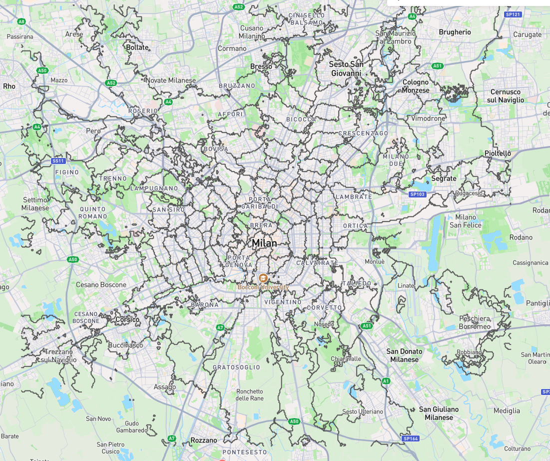
The resulting GeoJSON, showing the areas where a station is the quickest to reach
Not bad. Let’s zoom:
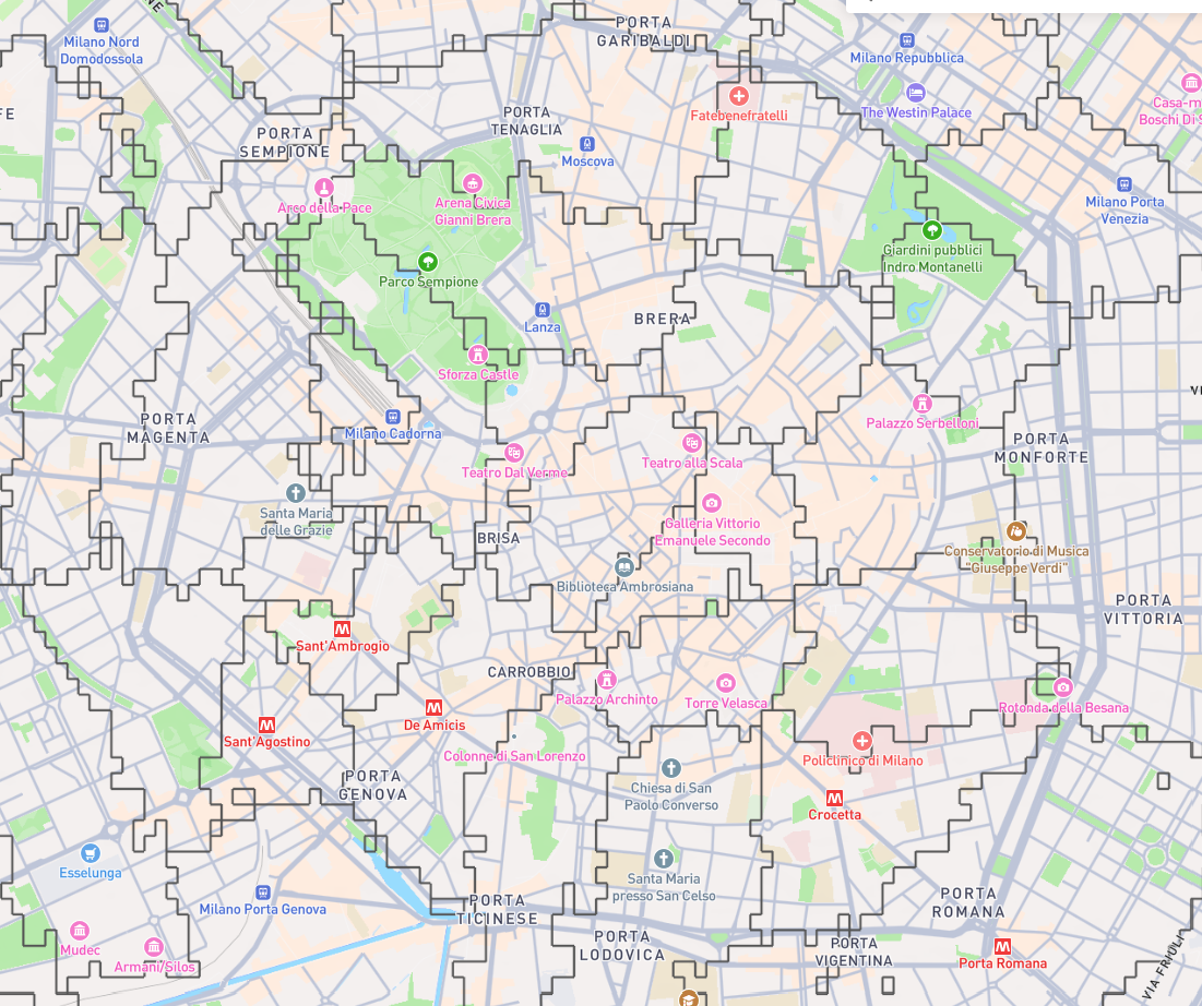
The resulting GeoJSON, zoomed
you can see that the regions are not contiguous and sometimes contains “islands” from others. This is due not only to calculation errors (e.g. incorrect tags on OSM or values r5py cannot recognize) but also due to the “non-linear” nature of public transport. A tram provides a quick connection from A to B, meaning that if B is close to a metro station and I’m closer to A by walk it will be easier to walk to it; if I’m not too close however it may be better to walk to a station, and the nearest by walk may be another one. This creates “islands” where the closest station is different than the one on surrounding points.
Another reason for these strange edges is the presence of fields and large buildings or areas without a clear walk network. When asked to calculate a route from these points r5py finds the closest road to start the graph navigation, which may be different depending on the position.
A nicer representation with Voronoi and Shapely
These edges are cool to see but not very usable: the geoJSON file is more than 6 MB and it contains no data about the name of the station. In fact it does not even know if a given point is closer to a station or another, because those edges are just isolated segments that happen to form shapes, but there’s no explicit “inside” or “outside” each region.
To handle this, I decided to explicitly find these regions.
My first idea was to use DuckDB again and extend the previous logic to expand a list of cells to
include their neighbors, using WITH RECURSIVE to perform a graph search and mark the regions.
Then I would have lists of cells that are in the same region, and would face the problem of
converting these cells to a closed polygon that can be displayed.
Another issue with this approach is that if later I add origin points that are not in an orthogonal grid (e.g. adding random points) I have no way to apply this logic.
I decided then to look at Voronoi, using the cells centers.
A Voronoi tessellation in 2D splits the plane into areas that are closest to a point in a given set of points. This is the approach used in the original Reddit post, but here I can use it not for the points representing the metro stations but rather on every point in the grid, which are orders of magnitude more.
Scipy provides a fast implementation of Voronoi, which doesn’t just provide the regions but also tracks which point is at the center of which region (if any, regions on the border are infinite).
With this function, I can get for each point in the grid the region (usually a rectangle) that surrounds it and is not closer to other points. This works even with random points added outside the grid pattern.
Iterating over these regions I generate Shapely Polygon objects and keep track of the nearest
metro station for each one. If you never heard of it, Shapely is THE Python library for 2D geometry,
performing pretty much everything you may need regarding points, polygons and the shapes you see on
a map. It is based on GEOS, the same library powering PostGIS.
Shapely can take a list of regions, in this case our cells, and aggregate them into a single polygon. This polygon effectively looses the detail of the internal regions and preserves only the external border which is what I want. Shapely also exports it as a GeoJSON, I only need some manipulation of it to add the name and color properties to each region.

The resulting GeoJSON, in a tool like gojson.io you can see the details about the station name and color are visible
this GeoJSON nicely handles disconnected regions too, they are just MultiPolygon objects.
Generate the heatmap
So far we were concerned only with the closest station, and used the travel time only to find it, but ignoring the actual time.
This data is however there to be used, and it can be represented with an heatmap.
There’s not much to say about it, I simply iterate over the cells and assign them a color based on the travel time. I then paint a rectangle of that color on a Pillow image.
For the color I used matplotlib colorscale, and decided to only consider travel tims lower than 40 minutes or the scale would be very unbalanced.
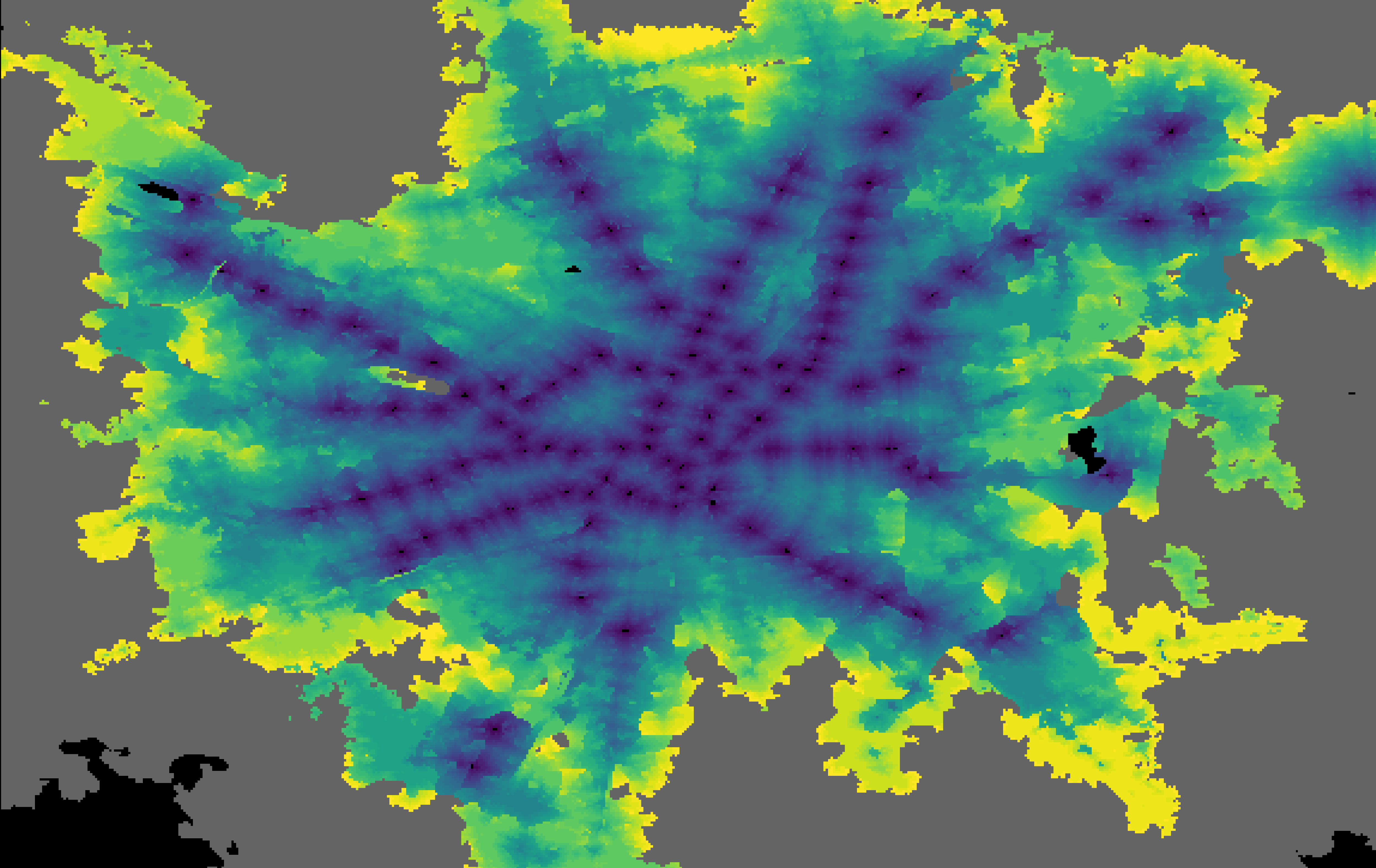
Heatmap of the travel time to the nearest metro station in Milan
Put it in the frontend
On the frontend I use the freshly released maplibre-gl 5.1, which adds a 3D globe functionality
(not that I need it at a city scale, but it sure looks cool), with a basemap from MapTiler.
With Maplibre is easy to load the geoJSON file as is and the heatmap image as a raster source, the Python script that generates the heatmap also provides a small JSON with the covered extent to correctly position the image on the map.
Done that, it’s just a matter of figuring out the best style, changing the width of the lines and
the colors. For example I noticed that the lilac color of the line M5 becomes too bland on the map
with a lower opacity so I replace it with #FC1FD0.
I tried to figure out an optimal opacity level for the overlays: too opaque and you can’t see the street names, too transparent and you can’t see the overlay itself. Eventually I just left a slider so the user can regulate it as they please. A few buttons allow the users to enable or disable the overlays altogether.