
Visualize the functioning of supervised learning models – part 2 – SVR and GridSearchCV
In the previous article we used a linear regression model to predict the color of an image pixel given a sample of other pixels, then used a hand-written function to enrich the coordinates and add non linearity, seeing how it improves the result. Without it, we can only get a gradient image.
Again, all the code is visible in the notebook.
I had fun playing with the enrichment function, but scikit-learn offers kernel methods out of the box. It uses a native implementation (libsvm), which is arguably faster than doing it in pure Python.
The code to train and use an SVR (Stochastic Vector Regression) is super simple:
from sklearn.svm import SVR
svr_rbf_red   = SVR(kernel='rbf', gamma=0.001)
svr_rbf_red.fit(X_train, Y_train[:, 0])
all_results_red = svr_rbf_red.predict(all_coordinates)
This is applied to a single channel (red), as the SVR does not support a different output shape than (N, 1). I trained and applied three models for three different channels, and only later discovered Scikit learn offers a MultiOutputRegressor which does exactly that…
However, the result is this:
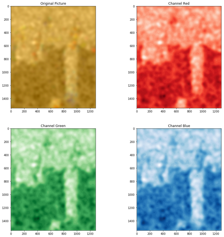
The result of an SVC model applied to the problem, with the RBF kernel and gamma=0.001
A strange issue is that the reconstructed image now is very dark and flat, pixel intensity on all channels goes from 42 to 103 (on the usual 0-255 range), so I adjusted it by subtracting the minimum and multiplying to cover the whole range 0-255. This luckily does not destroy colors too much but have yet to figure out the reason.
Above I used \(gamma=0.001\) as a parameter of the SVR model, and found it by trying different values and seeing the result. This parameter tells the kernel how much easily it can “bend”. If it’s too large, the model can overfit and wrap single samples without generalizing. If it’s too small, on the other hand, the model will have hard times learning the shape of the data. One needs to try different values to find an equilibrium.
The SVR model also has a \(C\) parameter. What the C parameter does is similar, as it sets a balance between overfitting and not modeling the data shape, but with respect to the margins of the hyperplane (or in this case, the curves generated by the kernel). The parameter tells the model how much to try to fit samples that are already inside the margin.
Since trying values by hand is annoying and error prone, scikit-learn also provides a tool called GridSearchCV to perform this operation automatically. It has the additional advantage of using multiple cores and train different models in parallel. And with Dask it can also exploit different machines of a cluster.
The code is this:
from sklearn.model_selection import GridSearchCV
X_train, Y_train, X_test, Y_test = extract_dataset(photo, train_size=2000, test_size=500)
parameters = {'kernel':['rbf', 'sigmoid'], 'C':np.logspace(np.log10(0.001), np.log10(200), num=20), 'gamma':np.logspace(np.log10(0.00001), np.log10(2), num=30)}
svr_red = svm.SVR()
grid_searcher_red = GridSearchCV(svr_red, parameters, n_jobs=8, verbose=2)
grid_searcher_red.fit(X_train, Y_train[:, 0].astype(float))
A part that gave me a few some headaches is the use of the logspace function: it enumerates values using the start and end values as exponents, not values for the range start and stop values themselves. So to have a range between, say, 1 and 10 one has to use 0 and 1. And yes, it uses base 10 by default instead of e.
The search lasted 10 minutes using 8 cores of an i7 processor, and examined 1200 candidates for each of the 3 channels, picking this one as the best:
SVR(C=55.33843058141432, cache_size=200, coef0=0.0, degree=3, epsilon=0.1, gamma=0.0001903526663201216, kernel=’rbf’, max_iter=-1, shrinking=True, tol=0.001, verbose=False)
the model is the same for all the channels (unsurprisingly), except the value of gamma for blue that was a bit lower (\(0.0001249\)), and the reconstructed image is this:
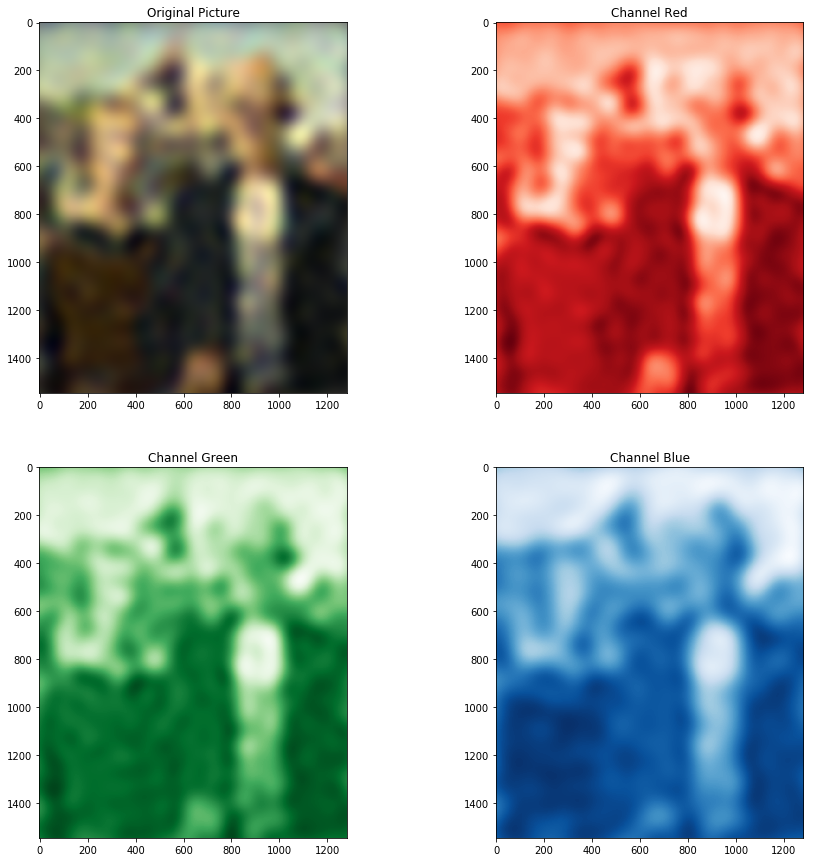
The image reconstructed by the SVR model picked by GridSearchCV
This time, the model predicted an image that was already balanced and needed no normalization.