
Visualize the functioning of supervised learning models
ConvnetJS offers a demo of a neural network which paints an image learning to predict the color of a pixel given its coordinates. I liked the idea as it is immediate and visually appealing, and decided to create a visual comparison of various supervised learning models applied to this toy problem. In this and further articles will review the results
All the code is in this Jupyter notebook.
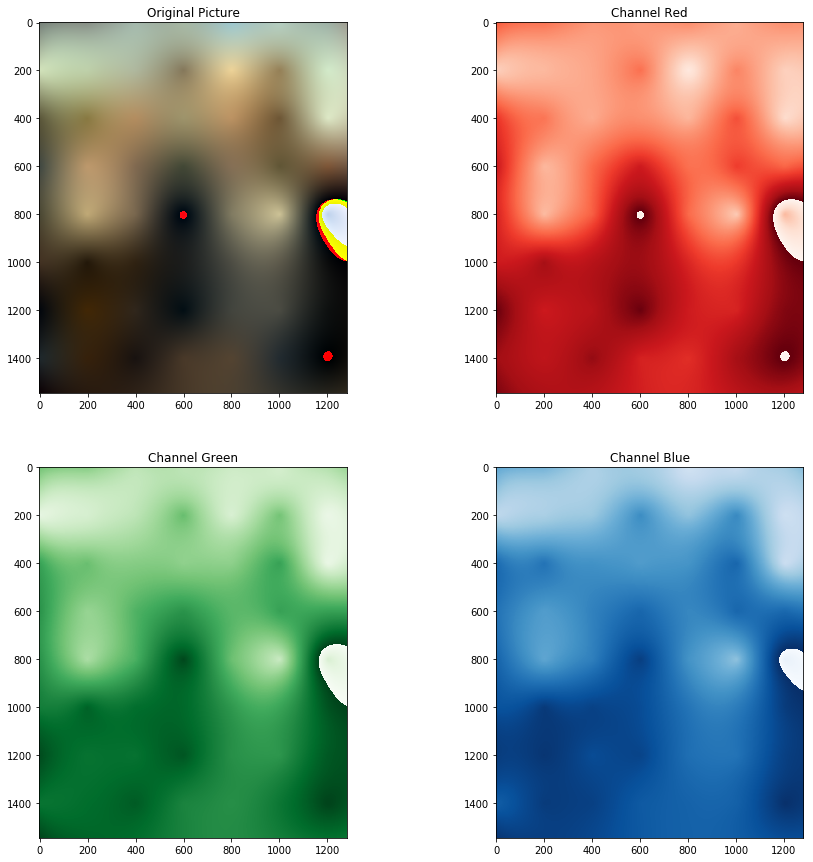
Given an image with the 3 RGB channels, a train and test dataset can be created just by sampling random pixels. The model can then be applied on all the coordinates to re-generate an approximation of the whole image and see how the model generalizes (or overfits).
This is the image:
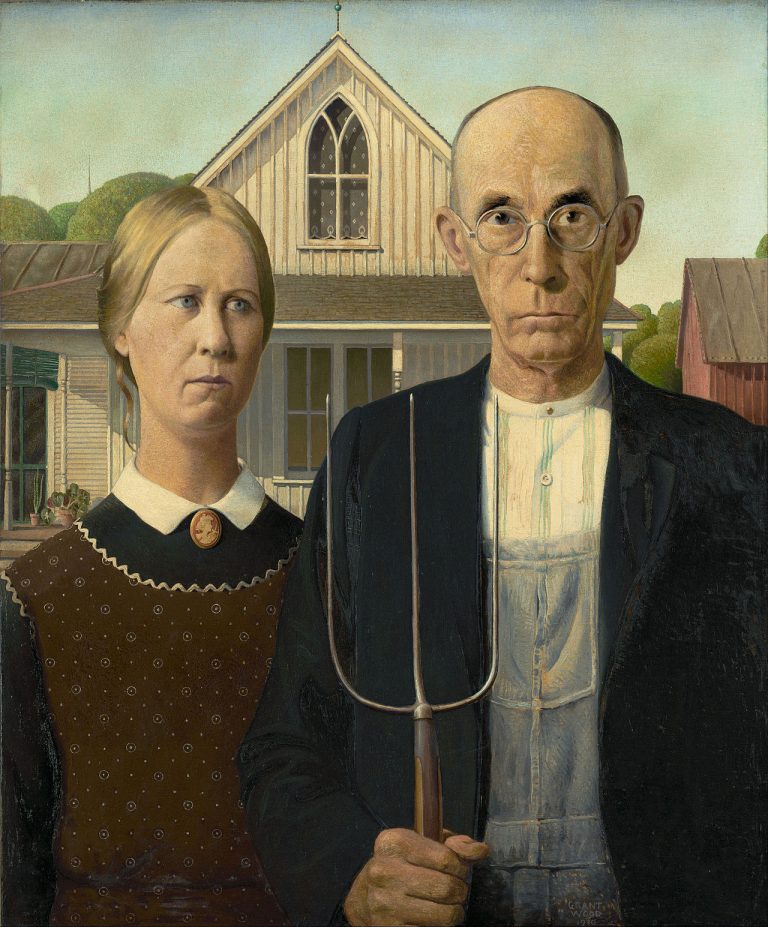
American Gothic by Grant Wood, from Google Art Project.
Linear model
The simplest model, linear regression, searches for the parameter of a linear function mapping \(Y=AX+b\), where \(X\) is the vector with the coordinates and \(Y\) one with the three colors of that pixel. In this case, the model parameters will define 3 planes for each channel, what in graphics is called gradient.
Scikit-learn provides this model and it calculates the exact solution given the training set instead of using gradient descent.
This is the result:
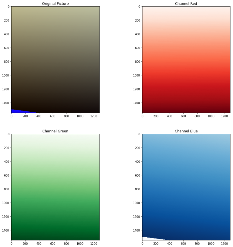
Gradients from the linear model
The small stains in the corner are negative values which overflow during the conversion of the matrix in uint8 that is necessary to avoid a bizarre behavior of matplotlib. The upper part of the image is brighter, and the model catches that, but that’s pretty much it.
To ensure that the model works, it is possible to test it on an image that is a gradient, which leads us to a dedicated Tumblr (?)
Gradients from the linear model
Gradients from the linear model
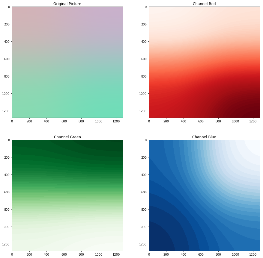
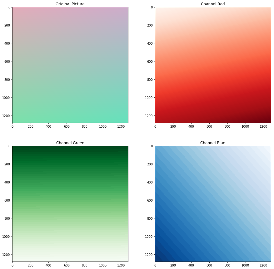
As expected the model worked well in this case. There’s a small difference on red and blue channels because the gradient apparently was not linear but radial, and in both cases there are artifacts due to quantization visible in the blue channel.
SVR – Support Vector Regression
To overcome the limit of the linear model, it is possible to “invent” new input dimensions by applying non-linear functions to the original ones, and training a linear model on this set of enriched dimensions. This is called kernel function and is commonly used in SVM models for classification. An SVR is Support Vector Machine applied to regression instead of classification.
I implemented a kernel function by hand because it’s interesting to be able to see how the result changes based on the function, but found there are many advantages one can exploit directly using libraries like scikit-learn: first, the kernel trick allows to reduce the computational effort when the kernel function follow certain properties. Then, it is easier to try different hyperparameters of the kernel function using tools like GridSearchCV. Using Dask that can be done in parallel with multiple machines.
def enricher(coordinates):
    ref_coordinates = list(itertools.product(np.arange(0, photo.shape[0], 200), np.arange(0, photo.shape[1], 200)))
    return [coordinates[0],
            coordinates[1],
           ] + [np.sqrt((coordinates[0] - p[0]) ** 2 + (coordinates[1] - p[1]) ** 2) for p in ref_coordinates]
This function adds to each coordinate a set of euclidean distances to some reference points. These reference points are arranged regularly in a grid.
The result of applying linear regression to the “enriched” coordinates using the kernel method
Much better! It is possible to distinguish some areas. There are again some artifacts due to negative values being casted to uint8.
In the next article I’ll delve more into the details of GridSearchCV and proper SVR using scikit-learn.