
Making a fully static map, part 2: Vector tiles
UPDATE: I created a Python tool to automate this process, including a refined style and packaging. I suggest using it.
In the previous post of this series we saw that an extract of the data from OpenStreetMap can be easily transformed into a set of raster tiles, essentially fragments of the map at different levels of zoom, arranged in a structure that enables a library like Leaflet.js to fetch them as needed when the user zooms and pans on the map.
NOTE: a complete demo of the final result is available on GitHub
This enables fully customized maps that don’t rely on external services and can be used as a base for data visualization, and interestingly makes possible to show historical snapshots of the map.
However, there are two disadvantages with this approach:
- raster images tend to consume a lot of space, we saw the city of Milan takes almost 4 GB.
- every change to the style of the map requires reprocessing, it cannot be applied later like CSS is to HTML.
the solution to both issues is to use vector tiles. In essence, instead of preprocessing the map data to render it, we only split it into chunks to allow random access to them, and let the browser do the rendering.
Imagine having a large lake, rendered as a blue area. With a raster representation, we have to produce completely monochromatic blue files for all the levels of zoom that don’t show anything but the water.
Zooming into an edge of a raster image will produce grainy pixelated artifacts, while on vector formats like SVG zooming is never a problem: the computer recalculates the colors on the screen based on the coordinates, you can zoom at will and will never be grainy.
This is the very basic principle of vector tiles, and to that we can add that if a file represents the semantic of the data then the client-side library has more flexibility in displaying it.
The file is essentially saying:
hey, here there’s a path marked as ‘street’ with this name and these ‘surface’, ‘bicycle’ and ’lit’ tags. Here is the list of coordinates of the points that make up this geometry: [45.5098864, 9.1942170], [5.5099752, 9.1938485]…
rather than
hey, here’s the color of the pixels: [ [34, 0, 89], [12, 45, 0], [0, 0, 255], [34, 0, 89], [12, 45, 0]…
so, more semantic. For a modern browser handling the vector data is not a problem.
Even better, we can represent this data in a binary format like protobuf to make it very fast to move around, and get small files.
Since we can zoom freely without artifacts, the tiles don’t need to be produced for high levels of zoom, saving up space and allowing the user to zoom at will.
The frontend, now, needs to know how to go from the geometry to the representation (e.g. if amenity=park then the area is green, or maybe not visible at all), the same operations that we previously implemented using QGIS styles.
In general, compared to raster, vector tiles:
- require less space on disk
- are faster to produce
- do not require reprocessing to change the style
- in fact, the style can be changed dynamically
- make the frontend aware of features (e.g. the user can click on a road or building and have it highlighted)
- can be zoomed without becoming pixelated
- enable 3D/perspective manipulation
All of this is possible using a format from Mapbox called Mapbox Vector Tile, widely adopted by FOSS and commercial tools.
MBTiles and vector tiles
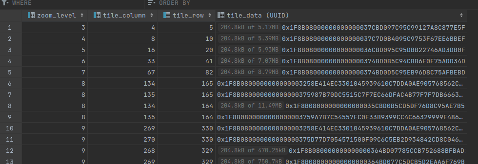
A possible source of confusion when dealing with this format is that there are two flavors. Many tools, including QGIS, offer to generate MBTiles, where MB stands for MapBox. The plural tiles may suggest this is a folder with vector tiles, like the one we generated with raster files. Instead, this is a SQLite database containing a table with zoom, column, row and tile data. The tile data can be raster or vector.
You can generate one using QGIS and the Write Vector Tiles (MBTiles) tool in the processing toolbox, and have a look at it with any SQLite client.
The content of an MBTiles file
the tile data itself is a blob of bytes, that is compressed with gzip and is ultimately using protobuf. Unlike the OSM export format, this is pure protobuf and can be examined using tools such as protoc.
In the same SQLite database we can see a metadata table, containing a list of the layers included in the file and, for each of them, the attributes and their types.
This can generate some confusion: an MBTiles file is indeed a single file that contains multiple tiles, not necessarily in vector format. It’s not a collection of files.
To serve a map in MBTiles format, then, you need a backend, albeit a simple one.
In my cas, I prefer to have single files so that I can keep using nginx to serve static files and not introduce a backend component to extract the single tiles.
Producing the tiles with Tilemaker
From an MBTiles generated by QGIS is trivial, using a bit of Python, to extract the tiles as single files. However, I prefer to use a separate tool called Tilemaker.
There are several reasons for this:
- The advantage of QGIS, the fact that we can see the map we are exporting, is lost here since we are exporting the raw data, not the style
- The QGIS tool tends to fail without clear errors (e.g. when no layer is selected)
- …however QGIS can generate the command to run it from the shell, in this case you get a meaningful error
- Tilemaker can be configured very extensively, even using Lua scripts to customize the export
The setup of Tilemaker can be tricky due to the dependencies, but a Dockerfile is provided and it helps a lot.
My procedure is as follow:
git clone https://github.com/systemed/tilemaker.git
# change the tilemaker/config.json file if needed
docker build tilemaker/. -t tilemaker
docker run --rm -it \
    -v /home/jacopo/projects/static-maps/:/opt/input \
    -v /home/jacopo/projects/static-maps/milano_protobuf_tiles:/opt/output \
    --user "$(id -u):$(id -g)" \
    tilemaker  --input /opt/input/milano.pbf --output /opt/output \
    --bbox 9.0,44.0,11.0,46.0
the --user flag is necessary to get the files created with the current user and not root (the default user in the container). Alternatively, run sudo chown -R $USER:$USER milano_protobuf_tiles afterwards to reassign them.
The --bbox flag specifies the coordinates of the area we want to process, and it is mandatory if they are not already specified in the PBF file. Creating the PBF from a larger file using Osmium you can add them using the --set-bounds flag, by default they are not set.
You can get the bounding box using osmium:
osmium fileinfo --extended filename.osm.pbf
Before building the Docker image I manipulate the config.json to:
- disable compression, or the PBF files will be gzipped
- …or keep it, but be sure to enable
gzip_staticin nginx
- …or keep it, but be sure to enable
- choose the layers to export, and at which zoom level they are visible
- this is to keep the tiles small, for example you don’t want to incorporate the city and state name when looking at buildings, or house numbers when looking at whole regions
- set the metadata to add to the export like the tile server address and the description
- these details can be changed later
if the gzip decompression is not set properly, you will see this error in the browser console:
Unimplemented type: 3
it’s a bit laconic, but what it means is that the library is trying to parse the compressed file as if it was raw protobuf data. Either decompress it or check your content-type headers.
The result of this operation is a folder similar to the raster one:
[...]

├── 7
│   └── 67
│       └── 45.pbf
├── 8
│   └── 134
│       └── 91.pbf
├── 9
│   ├── 268
│   │   ├── 182.pbf
│   │   └── 183.pbf
│   └── 269
│       ├── 182.pbf
│       └── 183.pbf
└── metadata.json
to compare with the previous example, the whole city of Milan takes 55MB rather than 3 GB without using compression. A great improvement! The generation of the files is also 1-2 orders of magnitude faster.
The metadata.json file contains, among other things, 3 essential details:
- the
boundsandzoomfor this data, used by clients to stitch different sources together and know when to even try to fetch the tiles - the URL for the tiles, with
{z},{x},{y}placeholders- this is the same logic used by Leaflet in the previous article, and you have to change it to your static server. It must be an absolute URL.
- the list of the layers and their tags and types. These are necessary to get an idea of the content and apply the style later
notice that so far we stored the raw map data in a format that is very accessible for the frontend, but didn’t specify any style. Like when you work with HTML and CSS, this is the structure and what we need is presentation.
Enter MapBox GLJS
Leaflet itself does not support vector tiles. There is however a plugin called Leaflet.VectorGrid to add this feature. Due to the nature of vector data, it’s possible to perform overzooming, that is, to set up a maximum level of zoom in the UI (called maxNativeZoom in the Leaflet configuration) greater than the zoom level for which the tiles were generated.
This functionality however seems a bit buggy, in my experiments I found that the image looks blurry/pixelated at high levels of zoom due to how the plugin works.
Another issue is the lack of WebGL. Leaflet as such is compatible even with Internet Explorer 7, but this means no hardware acceleration nor 3D or special effects. This is not a big deal for 2D maps, but prevent further tinkering with 3D addition which is a function I’d like to explore.
The good news is, Mapbox GLJS is a library that does exactly this. Not a shocker, since is made by the same company that defined the vector tiles format.
After Mapbox GL JS changed the license a fork called MapLibre Gl JS was created, which offers a drop-in replacement.
But wait, we are missing something. We need a style.
Style your map
Rather than connecting directly to a tile source, as done in the previous article, Mapbox expects the URL of a JSON file. This file contains the configuration of the whole map, which can be fairly complex and now goes beyond simply importing tiles.
First of all, this JSON can define multiple sources, both raster and vector, that can be stitched together covering different boundaries and zoom levels; for example you can use a coarse raster world map and a detailed regional vector map.
[...]
  "sources": {
    "openmaptiles": {
      "type": "vector",
      "url": "http://127.0.0.1:8000/metadata.json"
    },
[...]
this is how the data generated by Tilemaker can be used, simply by referring to the URL of the metadata.json, specifying it’s vector and assigning it a name, in this case openmaptiles. An advantage of this mechanism is that you can later switch to maps provided by external services (like MapBox or Maptiler) simply pointing to their JSON and including the account token.
From these sources one or more layers are built, each one has its own setting and is populated by one of the sources, and defines a style.
This is an example of a layer definition:
{
    "id": "landuse_residential",
    "type": "fill",
    "source": "openmaptiles",
    "source-layer": "landuse",
    "maxzoom": 8,
    "filter": [
        "==",
        "class",
        "residential"
    ],
    "paint": {
        "fill-color": {
            "base": 1,
            "stops": [
                [
                    9,
                    "hsla(0, 3%, 85%, 0.84)"
                ],
                [
                    12,
                    "hsla(35, 57%, 88%, 0.49)"
                ]
            ]
        }
    }
}
there is a lot to unpack here. The first lines are just specifying that this layer is called landuse_residential and the source is the layer “landuse” (in this case, a data layer, one defined in the metadata.json) of the vector source “openmaptiles” we defined earlier in the same file.
The maxzoom field specifies that this layer is not rendered with a zoom lower than 8, since residential areas need not to be marked when observing up close
The filter section here is defining a condition to what effectively constitute this layer, which is class == residential. More complex logic with boolean operators can be built.
Then, something intriguing: the paint property specifies the style, and for the fill-color rather than just give a color a scale is defined, based on the zoom.
In this video you can see the result (I used different colors to make it more visible):
this is something you can see done by many map services, to make the transition between levels of details smoother.
Text labels
Text labels are another part of the layer definition:
[...]
{
    "id": "road_label",
    "type": "symbol",
    "source": "openmaptiles",
    "source-layer": "transportation_name",
    "filter": [
        "all"
    ],
    "layout": {
        "symbol-placement": "line",
        "text-anchor": "center",
        "text-field": "{name:latin}",
        "text-font": [
            "OpenSans"
        ],
        [...]
here the field name:latin that is specified in metadata.json is used as a source for the strings to display. Many options for the precise display are provided.
Regarding fonts, if you use a text property then you must specify a value for glyphs. This is an URL containing the {fontstack} and {range}, for example http://127.0.0.1:8000/{fontstack}/{range}.pbf (again, this cannot be a relative address).
The fontstack property will be replaced with the name of the font, for example RobotoBold, while range refers to the Unicode code points, for example 0-255. When the client library needs to render text, it will call this URL with the proper font name and range (for languages like Chinese or Japanese will usually retrieve multiple blocks).
The fonts are in PBF format, which is based on Signed Distance Fields and was introduced first by Valve.
Mapbox provide fonts as a service (in which case the URL will point to a Mapbox endpoint including an user account), or you can host the fonts as static files like done with the tiles, simply using folders to represent the fontstack and range.
Style editors
As you can see, the JSON style definition is extremely powerful, so powerful in fact that it can be overwhelming. You can even add some 3D effect using the extrusion property!
For this reason, just like we did with QGIS, you can use existing themes or tools to edit them. See Maputnik for an editor, the result can be exported as JSON ready to use.
Alternatively, services like Mapbox include an editor that publishes the style JSON at a given URL, directly updating the look of the map.