
Visualize the functioning of supervised learning models – part 4: Neural networks
After trying regression using k-neighbours, linear and SVR models, I wanted to conclude using neural networks.
I did the 5 deep learning courses from Andrew Ng on Coursera to get a grasp of these models, and decided to use Keras. This library makes defining, training and applying a model quite easy, once one has an idea of what to use.
Artificial neural networks
The naming is suggestive and one may think the goal is to replicate the human brain, but it’s more akin to a generic and very flexible mathematical function.
An artificial feed-forward neural network is basically a combination of smaller units called neurons, which themselves are just functions that receive a vector as an input, do a dot product with their own weights vector, apply a non-linear monotonic function called activation function and produce an output that goes to another neuron until the last layer of neurons (the output layer) which calculates the final output of the whole network.
This structure can be trained by giving it samples, observing the output, comparing it with the desired output to get the error, and slightly changing the weights of the network in proportion to the gradient of the error calculated for each weight; sample after sample the weights are increased or decreased to reduce the error in order to have the network “learn” from the samples and hopefully give a useful output once presented with a never seen input. This is called backpropagation, the name comes from the fact the forward propagation is the calculation of the output and this one goes backwards to “fix” a bit the weights which produced that output.
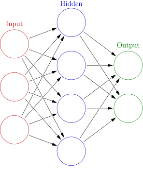
An artificial feed-forward neural network, every circle is a neuron (Source: Wikipedia)
These ideas are not new but in the last years (roughly after 2012) a new class of methods called deep learning attracted the attention of the vast public with some impressive breakthroughs in image recognition, automatic translation and other tasks. These methods use the parallelism offered by modern hardware (and in particular the GPUs) to apply huge neural networks with many, many layers (hence the term deep) to equally humongous datasets. Moreover, these models take advantage of many fancy variations on the mentioned model: by adding convolution to process images, “unrolling” a network to deal with sequences of varying length.
There is a lot of fascinating material around, so I’ll not say more. Just be aware that while there are many applications and is worth giving deep learning a look there is also much hype on the topic which in my opinion is leading to a new AI winter, and unless there’s scientific literature suggesting otherwise I think it’s better to start from simpler models when dealing with a new problem. The computational effort is lower and one is more likely to understand what the model is doing.
That being said, I wanted to try a simple FFANN (feed-forward artificial neural network) on my toy problem, which is not deep at all since the dataset is too small to exploit deep learning.
As usual, the whole code is in the notebook.
The model
First import the model and define a few constants:
from keras.models import Sequential
from keras.layers import Dense, Dropout
import numpy as np

N_NEURONS = 1000
ACTIVATION='selu'
I use 1000 neurons per layer, which is quite a lot for this case, and the selu activation function. There’s no easy way to choose the activation functions to use in the network, usually for classification a softmax is used on the output layer, linear activation in a layer can be nice for regression, but the general rule is to try them all and see what happens, or find someone who did and published the results.
A dense layer is one where all the neurons receive all the outputs of the ones in the previous layer. A dropout layer is a sort of filter which randomly disables 1% of the neurons at every iteration (both in forward and backward propagation). This is done to contrast overfitting.
Then, I define the network:
model = Sequential()
model.add(Dense(N_NEURONS, input_shape=(2,), activation=ACTIVATION))
model.add(Dropout(0.01))
model.add(Dense(N_NEURONS, input_shape=(N_NEURONS,), activation=ACTIVATION))
model.add(Dropout(0.01))
model.add(Dense(N_NEURONS, input_shape=(N_NEURONS,), activation=ACTIVATION))
model.add(Dense(3, input_shape=(N_NEURONS,), activation=ACTIVATION))
model.compile(optimizer='adam', loss='mse')
Easy, isn’t it? The last line compiles the model, so Keras transforms it into something we can actually use. I also define the Adam optimizer, which adds adaptive momentum to the backpropagation. This means that when iterating over samples the network will not just change weights proportionally to the error but also based on the error on previous iterations; empirically, it works well.
Then, the training:
X_train, Y_train, X_test, Y_test = extract_dataset(photo,
        train_size=5000, test_size=0)

model.fit(x=X_train, y=Y_train, epochs=400)
400 epochs is a lot, but this is a weird use case and trying different configurations found this works well.
The interface for fit and predict is identical to scikit-learn, I assume it is by purpose, and it wants the array of input and output samples.
Notably, Keras also allows to pass a generator which I really like using the fit_generator method.
Training the model doesn’t take long, and the prediction is simple as well:
all_coordinates = np.array(list(itertools.product(np.arange(predicted.shape[0]),
                                                np.arange(predicted.shape[1]))))
all_results = model.predict(all_coordinates)
This is the result:
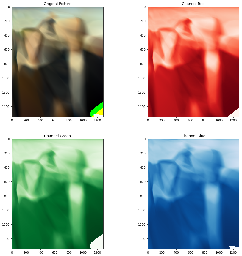
American Gothic reconstructed by the neural network